Relation between Schrödinger's equation and the path integral formulation of quantum mechanics

This article relates the Schrödinger equation with the path integral formulation of quantum mechanics using a simple nonrelativistic one-dimensional single-particle Hamiltonian composed of kinetic and potential energy.

1 Background
- 1.1 Schrödinger's equation
- 1.2 Path integral formulation
2 From Schrödinger's equation to the path integral formulation
3 References

Background

Schrödinger's equation

Schrödinger's equation, in bra-ket notation, is

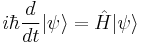
$i\hbar {d\over dt} |\psi\rangle = \hat H |\psi\rangle$

where $\hat H$ is the Hamiltonian operator. We have assumed for simplicity that there is only one spatial dimension.

The Hamiltonian operator can be written

$\hat H = {\hat{p}^2 \over 2m} %2B V(\hat q )$

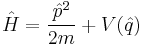
where $V(\hat q )$ is the potential energy, m is the mass and we have assumed for simplicity that there is only one spatial dimension q.

The formal solution of the equation is

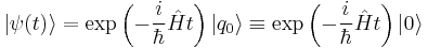
$|\psi(t)\rangle = \exp\left({- {i \over \hbar } \hat H t}\right) |q_0\rangle \equiv \exp\left({- {i \over \hbar } \hat H t}\right) |0\rangle$

where we have assumed the initial state is a free-particle spatial state $|q_0\rangle$ .

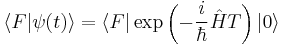
The transition probability amplitude for a transition from an initial state $|0\rangle$ to a final free-particle spatial state $| F \rangle$ at time T is

$\langle F |\psi(t)\rangle = \langle F | \exp\left({- {i \over \hbar } \hat H T}\right) |0\rangle$ .

Path integral formulation

The path integral formulation states that the transition amplitude is simply the integral of the quantity

$\exp\left( {i\over \hbar} S \right)$

over all possible paths from the initial state to the final state. Here S is the classical action.

The reformulation of this transition amplitude, originally due to Dirac^[1] and conceptualized by Feynman,^[2] forms the basis of the path integral formulation.^[3]

From Schrödinger's equation to the path integral formulation

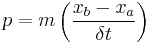
Note: the following derivation is heuristic (it is valid in cases in which the potential, $V(q)$ , commutes with the momentum, $p$ ). Following Feynman, this derivation can be made rigorous by writing the momentum, $p$ , as the product of mass, $m$ , and a difference in position at two points, $x_a$ and $x_b$ , separated by a time difference, $\delta t$ , thus quantizing distance.

$p = m \left(\frac{x_b - x_a}{\delta t}\right)$

Note 2: There are two errata on page 11 in Zee, both of which are corrected here.

We can divide the time interval from 0 to T into N segments of length

$\delta t = {T \over N}$ .

The transition amplitude can then be written

$\langle F | \exp\left({- {i \over \hbar } \hat H T}\right) |0\rangle = \langle F | \exp\left( {- {i \over \hbar } \hat H \delta t} \right) \exp\left( {- {i \over \hbar } \hat H \delta t} \right) \cdots \exp\left( {- {i \over \hbar } \hat H \delta t} \right) |0\rangle$ .

We can insert the identity

$I = \int dq |q\rangle \langle q |$

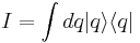
matrix N-1 times between the exponentials to yield

$\langle F | \exp\left({- {i \over \hbar } \hat H T}\right) |0\rangle = \left( \prod_{j=1}^{N-1} \int dq_j \right) \langle F | \exp\left( {- {i \over \hbar } \hat H \delta t} \right) |q_{N-1}\rangle \langle q_{N-1} | \exp\left( {- {i \over \hbar } \hat H \delta t} \right) |q_{N-2}\rangle \cdots \langle q_{2} | \exp\left( {- {i \over \hbar } \hat H \delta t} \right) |0\rangle$ .

Each individual transition probability can be written

$\langle q_{j%2B1} | \exp\left( {- {i \over \hbar } \hat H \delta t} \right) |q_j\rangle = \langle q_{j%2B1} | \exp\left( {- {i \over \hbar } { {\hat p}^2 \over 2m} \delta t} \right) \exp\left( {- {i \over \hbar } V \left( q_j \right) \delta t} \right)|q_j\rangle$ .

We can insert the identity

$I = \int { dp \over 2\pi } |p\rangle \langle p |$

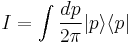
into the amplitude to yield

$\langle q_{j%2B1} | \exp\left( {- {i \over \hbar } \hat H \delta t} \right) |q_j\rangle = \exp\left( {- {i \over \hbar } V \left( q_j \right) \delta t} \right) \int { dp \over 2\pi } \langle q_{j%2B1} | \exp\left( {- {i \over \hbar } { { p}^2 \over 2m} \delta t} \right) |p\rangle \langle p |q_j\rangle$

$= \exp\left( {- {i \over \hbar } V \left( q_j \right) \delta t} \right) \int { dp \over 2\pi } \exp\left( {- {i \over \hbar } { { p}^2 \over 2m} \delta t} \right) \langle q_{j%2B1} |p\rangle \langle p |q_j\rangle$

$= \exp\left( {- {i \over \hbar } V \left( q_j \right) \delta t} \right) \int { dp \over 2\pi } \exp\left( {- {i \over \hbar } { { p}^2 \over 2m} \delta t} -{i\over \hbar} p \left( q_{j%2B1} - q_{j} \right) \right)$

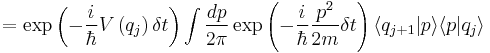
where we have used the fact that the free particle wave function is

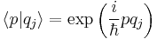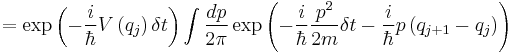
$\langle p |q_j\rangle = \exp\left( {i\over \hbar} p q_{j} \right)$ .

The integral over p can be performed (see Common integrals in quantum field theory) to obtain

$\langle q_{j%2B1} | \exp\left( {- {i \over \hbar } \hat H \delta t} \right) |q_j\rangle = \left( {-i m \over 2\pi \delta t } \right)^{1\over 2} \exp\left[ {i\over \hbar} \delta t \left( {1\over 2} m \left( {q_{j%2B1}-q_j \over \delta t } \right)^2 - V \left( q_j \right) \right) \right]$

The transition amplitude for the entire time period is

$\langle F | \exp\left( {- {i \over \hbar } \hat H T} \right) |0\rangle = \left( {-i m \over 2\pi \delta t } \right)^{N\over 2} \left( \prod_{j=1}^{N-1} \int dq_j \right) \exp\left[ {i\over \hbar} \sum_{j=0}^{N-1} \delta t \left( {1\over 2} m \left( {q_{j%2B1}-q_j \over \delta t } \right)^2 - V \left( q_j \right) \right) \right]$ .

If we take the limit of large N the transition amplitude reduces to

$\langle F | \exp\left( {- {i \over \hbar } \hat H T} \right) |0\rangle = \int Dq(t) \exp\left[ {i\over \hbar} S \right]$

where S is the classical action given by

$S = \int_0^T dt L\left( q, \dot{q} \right)$

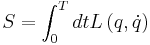
and L is the classical Lagrangian given by

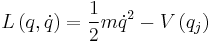$L\left( q, \dot{q} \right) = {1\over 2} m {\dot{q}}^2 - V \left( q_j \right)$ .

The integral

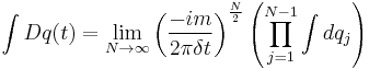
$\int Dq(t) = \lim_{N\to\infty}\left( {-i m \over 2\pi \delta t } \right)^{N\over 2} \left( \prod_{j=1}^{N-1} \int dq_j \right)$

is an integral over all possible paths the particle may take in going from its initial state to its final state. This expression actually defines the manner in which the path integrals are to be taken. The coefficient of the integral is a normalization factor and has no significance.

This recovers the path integral formulation from Schrödinger's equation.

References

^ Dirac, P. A. M. (1958). The Principles of Quantum Mechanics, Fourth Edition. Oxford. ISBN 0-19-851208-2.
^ Richard P. Feynman (1958). Feynman's Thesis: A New Approach to Quantum Theory. World Scientific. ISBN 981-256-366-0.
^ A. Zee (2003). Quantum Field Theory in a Nutshell. Princeton University. ISBN 0-691-01019-6.